One Hundredth of a Second

A Bayesian forward simulation of aerodynamic drag at the 1980 Olympics

Kristian Vepsäläinen

2026-07-01

One hundredth
of a second.

Lake Placid, 17 February 1980

Kristian Vepsäläinen · useR! 2026

The race

Men’s 15 km cross-country skiing

Gold: Thomas Wassberg 41:57.63
Silver: Juha Mieto 41:57.64

Δ = 0.01 s

After 42 minutes of skiing, one hundredth of a second. FIS changed its timing rules. Cross-country times are now rounded to 0.1 s.

The folk theory. Juha Mieto had a beard. For decades Finnish skiing folklore has asked: did it cost him the gold?

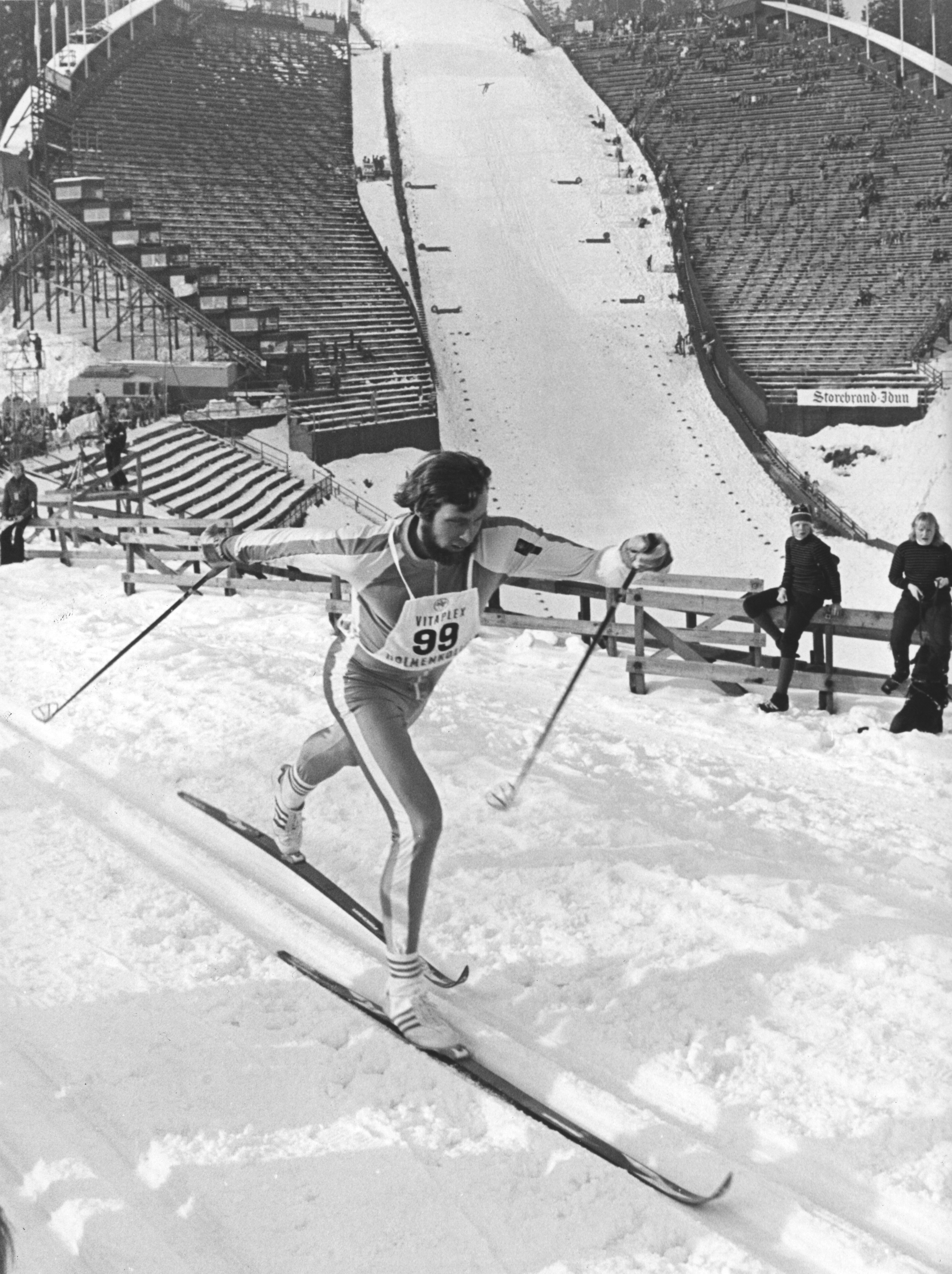
Juha Mieto at the Holmenkollen Ski Festival, 1978. DEXTRA Photo / Norsk Folkemuseum · Wikimedia Commons · CC BY

This is not a history talk

We cannot know what happened on 17 February 1980.

We can ask a different, sharper question:

Under physically plausible assumptions, is 0.01 s a typical outcome of additional aerodynamic drag, or an extreme one?

This is a modeling question — and it is exactly the kind of question R is good at.

Why this is a useR talk

This is a story about three things every applied modeller meets:

Sparse data. We have three split times. That’s it.
Unknown nuisance parameters. Course profile, wind, body shape, power output.
A claim about a small margin. “Negligible” vs. “plausible” — who decides?

The toolkit:

Bayesian forward simulation + R + honest priors + a single plot.

The plan

1. Physics

A drag-power model of cross-country skiing.

Frontal area · drag coefficient · velocity³ · power.

2. Priors

Honest, wide, defensible ranges for every unknown.

Not point estimates.

3. Propagate

100,000 simulated races.

Look at the posterior of the time loss attributable to drag.

No Stan. No JAGS. Just runif, rnorm, and a loop.

What we know

Three split times for Juha Mieto (sports-reference.com archive)

Distance	Cumulative time	Split speed
5 km	13:25.00	6.21 m/s
10 km	25:51.97	6.70 m/s
15 km	41:57.64	5.18 m/s

Venue: Mt. Van Hoevenberg, Lake Placid, NY. The trails still exist.

Everything else is a prior.

The physics

The power needed to overcome aerodynamic drag:

\[ P_\text{drag} \;=\; \tfrac{1}{2}\,\rho\,C_d\,A\,v^{3} \]

Symbol	Meaning	Treatment
\(\rho\)	Air density	Fixed at 1.2 kg/m³
\(C_d\)	Drag coefficient (body)	Prior: U(0.7, 0.9)
\(A\)	Frontal area (body)	Fixed at 0.5 m²
\(A_\text{beard}\)	Additional frontal area from beard	Prior: U(0.005, 0.015) m²
\(v\)	Local velocity	Derived from splits + terrain
\(P\)	Total power output	Prior: N(400, 30) W

The beard adds frontal area. The body still has to push through air. \(\Delta P = \tfrac{1}{2}\rho C_d A_\text{beard} v^3 \cdot \alpha^{3}\) where \(\alpha < 1\) accounts for slipstream shielding.

Anchoring v to the split times

The splits give us average segment speeds. We don’t know how the speed was distributed within each segment.

So we model it:

profile     <- c(up = 0.4, flat = 0.3, down = 0.3)   # course mix
speed_mult  <- c(up = 0.7, flat = 1.0, down = 1.3)   # relative speeds

for (k in 1:3) {                                      # for each split
  v_obs <- v_segments[k]
  scale <- v_obs / sum(profile * speed_mult)          # match the split
  for (seg in names(profile)) {
    v <- rnorm(N, speed_mult[seg] * scale, 0.2)       # local v
    v[v < 1] <- 1
    v3_mean <- v3_mean + profile[seg] * v^3           # accumulate E[v³]
  }
}

Jensen’s inequality matters: drag depends on \(\mathbb{E}[v^3]\), not \(\mathbb{E}[v]^3\). Modelling within-segment variation is not optional.

The priors, visualized

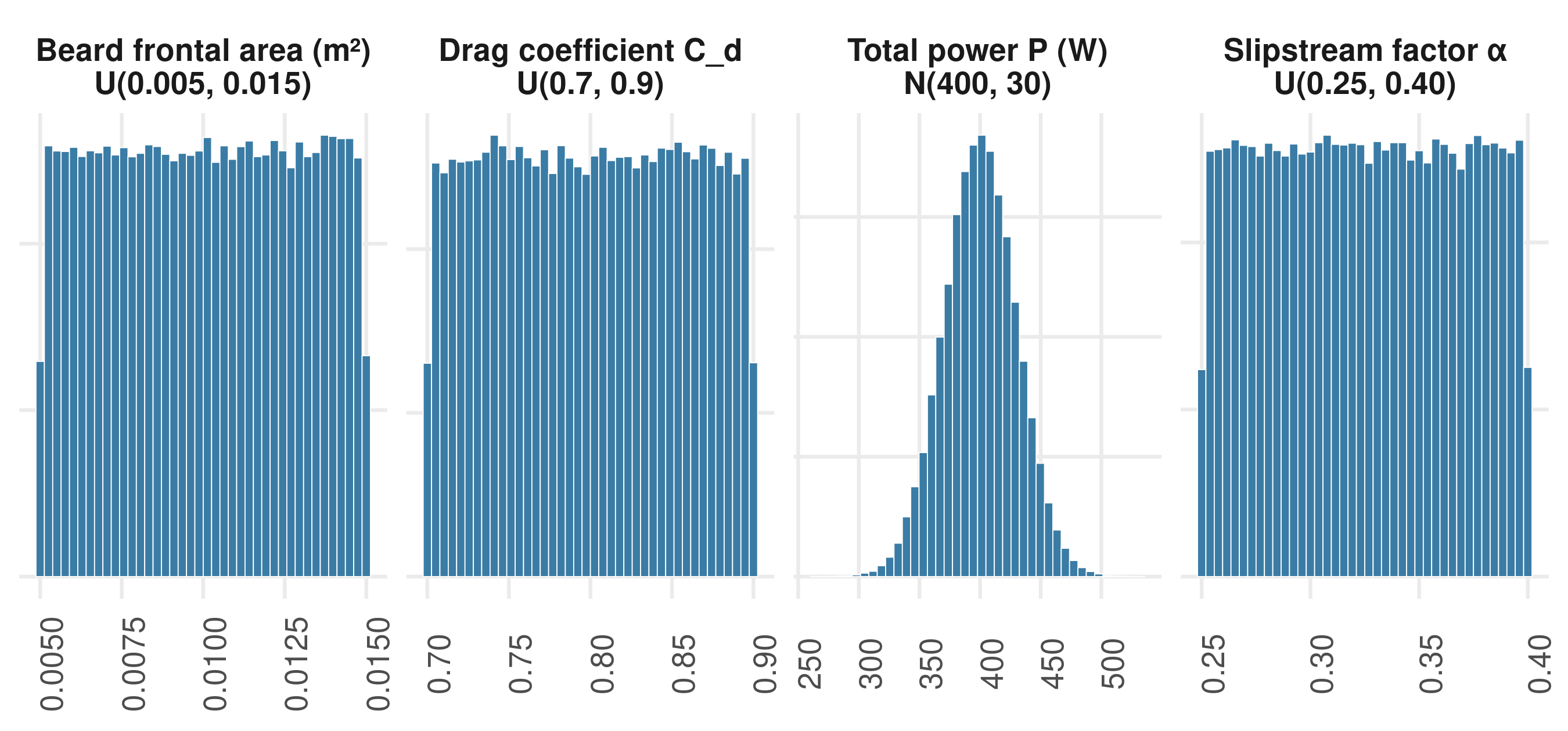
Wide on purpose. The goal is to ask: does the conclusion survive honest uncertainty? — not to pretend we have a tight estimate.

The model — one screen of R

set.seed(1980)
N <- 100000;  rho <- 1.2;  A_body <- 0.5
T_total <- 41*60 + 57.64

v_segments <- c(5000 / (13*60 + 25.00),
                5000 / ((25*60 + 51.97) - (13*60 + 25.00)),
                5000 / ((41*60 + 57.64) - (25*60 + 51.97)))

profile    <- c(up = 0.4, flat = 0.3, down = 0.3)
speed_mult <- c(up = 0.7, flat = 1.0, down = 1.3)

A_beard <- runif(N, 0.005, 0.015)
Cd_body <- runif(N, 0.7, 0.9)
P_total <- rnorm(N, 400, 30)
alpha   <- runif(N, 0.25, 0.40)

v3_mean <- numeric(N)
for (k in 1:3) {
  v_obs <- v_segments[k]
  scale <- v_obs / sum(profile * speed_mult)
  for (seg in names(profile)) {
    v <- rnorm(N, speed_mult[seg] * scale, 0.2);  v[v < 1] <- 1
    v3_mean <- v3_mean + profile[seg] * v^3
  }
}
v3_mean <- v3_mean / 3

P_drag_body  <- 0.5 * rho * Cd_body * A_body * v3_mean
P_drag_beard <- P_drag_body * (A_beard / A_body) * alpha^3
delta_time   <- T_total * (P_drag_beard / P_total)

p_active        <- runif(N, 0.05, 0.20)   # fraction of race in beard-exposed posture
delta_time_real <- delta_time * p_active

The result

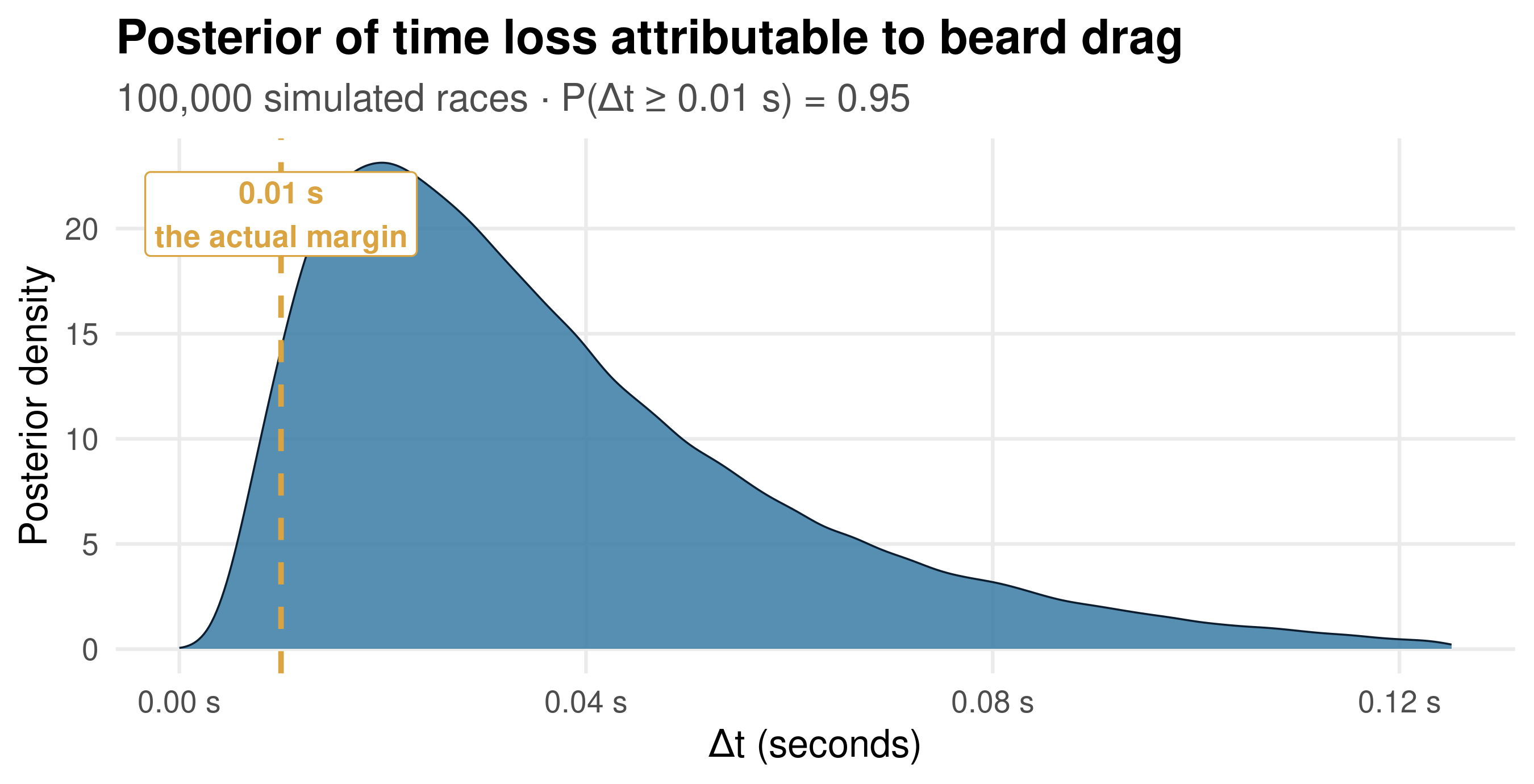
0.01 s is well inside the bulk of the distribution.

What the plot says — and doesn’t say

What it says

A margin of 0.01 s is not anomalous under physically plausible drag assumptions.

The folk theory is not absurd. It is consistent with the physics.

What it does NOT say

The beard caused Mieto to lose.

We have no counterfactual race without the beard. We have a distribution of plausible drag-time costs.

The right Bayesian sentence: “0.01 s is consistent with this model.” The wrong one: “the beard cost him gold.”

The general lesson

This is a template for a very common task in applied data science:

You have a small effect.
Someone tells you it is “negligible.”
You have no clean experiment available.
You have physics, plausible ranges, and R.

Forward simulation lets you ask:

Is the observed effect within the distribution of outcomes that the system can plausibly produce?

You don’t need a posterior over parameters. You need a posterior over consequences.

Where this approach earns its keep

Domain	“Negligible” effect	Forward simulation question
Finance	A 2 bp execution slippage	What return distribution would erase it?
Compliance	A rule threshold tweak	How many flagged cases shift, plausibly?
Manufacturing	A 0.1 °C drift	Yield consequence under realistic load?
Healthcare	A 1 % adherence change	Population-level outcome distribution?
Sports	0.01 s	Drag, wax, draft, terrain — which matters?

Every row is the same R script with different priors.

Why R, specifically

The model fits on one screen.

runif, rnorm, a for loop, ggplot2.
No probabilistic programming framework needed for the forward pass.
Reviewers can read it in 30 seconds.

The plot is the argument.

geom_density + geom_vline = the entire claim.
Reproducible from one .qmd file.
Priors visible, code visible, conclusion visible.

Transparency is the deliverable. The number is secondary.

Honest limitations

Course profile is a proxy. The 1980 Mt. Van Hoevenberg trail is approximated by today’s terrain mix (40/30/30).
Weather is assumed calm. Wind would dominate any beard effect.
The alpha slipstream factor is a back-of-envelope shielding estimate, not a CFD result.
p_active — the fraction of the race in beard-exposed posture — is the weakest prior.
No correlation structure between the four uncertain parameters.

Every one of these is a knob. Every knob is a runif(...) away from being tested.

Extensions (homework, if you like)

Sensitivity analysis: which prior moves \(P(\Delta t \geq 0.01\,s)\) most?
Replace runif with empirical distributions for \(C_d\) from wind-tunnel literature.
Add wind. A 1 m/s headwind dwarfs the beard.
Add Wassberg. Two skiers, two posteriors, one difference distribution.
Hierarchical version: pool across the four cross-country events at Lake Placid.

All of this is plain R. None of it requires more than 100 lines.

Takeaways

Forward simulation is underused. When data is sparse but physics is known, simulate first, fit later.
A prior is a hypothesis. Wide priors are not weakness — they are an honest test of robustness.
The plot is the argument. A single density with a single dashed line settled a 46-year-old question.

A negligible margin is only negligible relative to a model.

Thank you.