---
title: "What 56,000 Statutes Reveal About How a Country Legislates"
subtitle: "A reproducible analysis of Finnish legislation using open data and Bayesian methods"
author: "Kristian Vepsäläinen"
date: last-modified
execute:
echo: true
warning: false
message: false
cache: true
---
::: {.callout-note appearance="simple"}
**Download:** [PDF version](finlex-whitepaper.html) · [Source on GitHub](https://github.com/KristianVepsalainen/KristianVepsalainen.github.io/blob/main/whitepapers/finlex-whitepaper.qmd)
:::
```{r setup}
#| include: false
library(dplyr)
library(ggplot2)
library(fst)
library(tidyr)
library(here)
# Data is fetched and cached locally; see "Reproducing this analysis" below.
df <- read_fst(here("data","finlex","finlex_saadokset.fst"))
rik <- read_fst(here("data","finlex","finlex_rikastettu.fst"))
aff <- read_fst(here("data","finlex","finlex_affected.fst"))
VUOSI_ALO <- 1987
VUOSI_LOP <- 2024
df_a <- df |> filter(vuosi >= VUOSI_ALO, vuosi <= VUOSI_LOP)
rik_a <- rik |> filter(vuosi >= VUOSI_ALO, vuosi <= VUOSI_LOP)
fmt <- function(x) formatC(as.integer(x), format = "d", big.mark = ",")
n_total <- nrow(df_a)
```
## The question
Every lawyer knows what the law *says*. Almost nobody knows how the law *behaves* as a system — how fast it changes, which parts change most, when in the year new rules appear, or whether the pace of new legislation is rising or falling. These are empirical questions, and the data to answer them is public.
This whitepaper demonstrates a reproducible pipeline that turns Finland's open legislative database into quantitative answers. It is written for two audiences: data professionals who want to see the method, and decision-makers who want to know what kind of insight open legal data can deliver. The same approach generalises to any jurisdiction that publishes machine-readable legislation.
All code is shown. All figures are computed from the data, not hard-coded. The entire analysis rests on `r fmt(n_total)` statutes retrieved from a free, public API.
## The data source
Finland publishes its legislation through an open REST API following the [Akoma Ntoso](http://www.akomantoso.org/) standard — a UN-backed XML schema for legal documents. No registration or API key is required; the only requirement is a `User-Agent` header.
Each statute carries a category — new statute, amending statute, or repealing statute — which is the key to most of the analysis. A statute is not a static text but an event: a law is enacted once and then amended, sometimes dozens of times, over its lifetime.
```{r fetch-demo}
#| eval: false
library(httr)
library(jsonlite)

BASE <- "https://opendata.finlex.fi/finlex/avoindata/v1/akn/fi/act/statute/list"
UA   <- "FinlexAnalysis/1.0 (your.email@example.com)"

# One page of results for a given year and category
fetch_page <- function(year, category, page) {
  resp <- GET(BASE,
    query = list(format = "json", page = page, limit = 10,
                 sortBy = "dateIssued",
                 startYear = year, endYear = year,
                 categoryStatute = category),
    add_headers(`User-Agent` = UA, Accept = "application/json"),
    timeout(30))
  stop_for_status(resp)
  fromJSON(rawToChar(resp$content))
}
```
The API caps page size at ten results and returns both Finnish and Swedish language versions, so the full retrieval loops over years and categories, keeps only the `fin@` URIs, and paginates until a page comes back empty. Retrieving the complete dataset of `r fmt(n_total)` statutes plus their amendment targets is an overnight job — roughly 90,000 HTTP requests in total. The retrieval code is built to resume from an interruption and to back off on HTTP 429 responses, which matters when a job runs for hours.
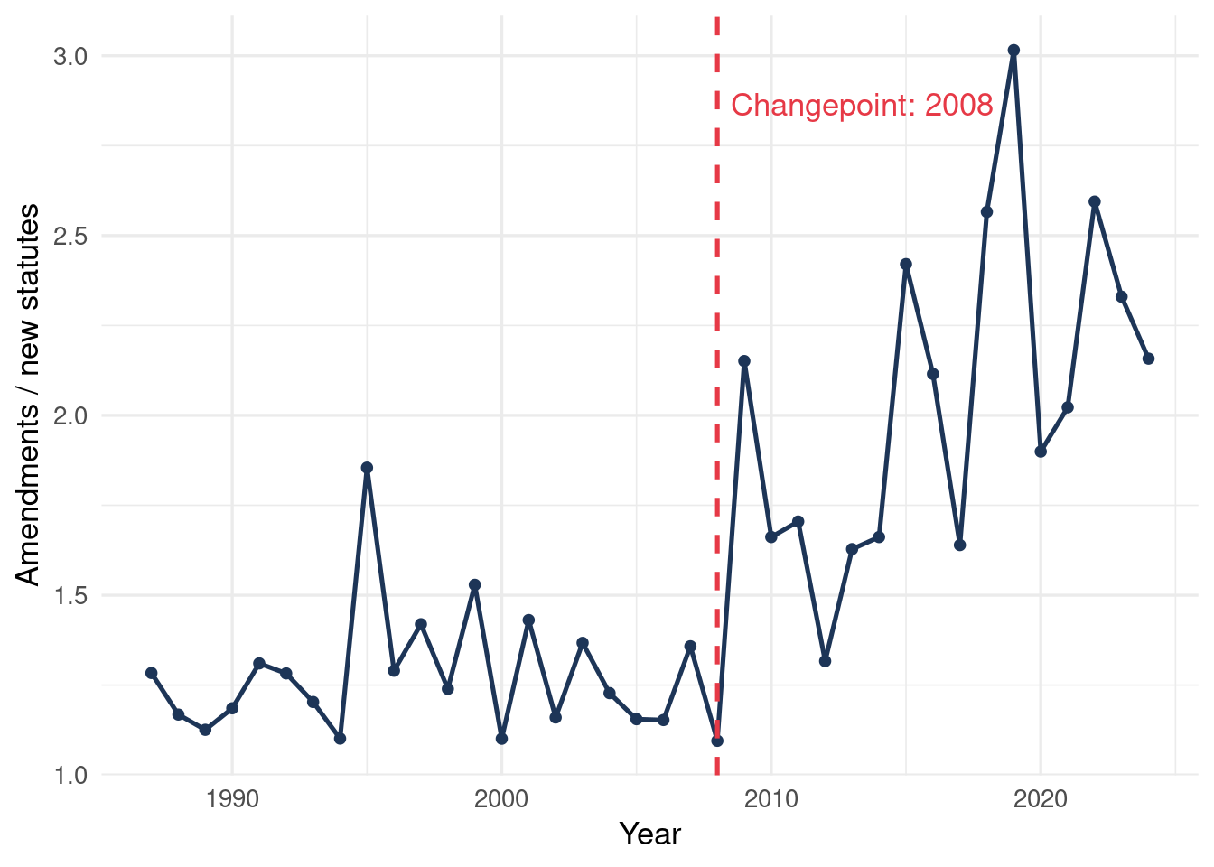
## Finding 1: EU membership left a measurable mark
The clearest structural signal in Finnish legislation is the ratio of amendments to new statutes — how much existing law is being modified relative to how much new law is created.
```{r changepoint-data}
ratio_data <- df_a |>
  count(vuosi, statute_type) |>
  pivot_wider(names_from = statute_type, values_from = n, values_fill = 0) |>
  mutate(ratio = Amendment / NewStatute) |>
  arrange(vuosi)
```
A Bayesian changepoint analysis locates the moment this ratio shifted. The method models the series as having one structural break at an unknown point, places a uniform prior over all possible break years, and marginalises to get a posterior distribution over the changepoint location — not a point guess, but a full description of the uncertainty.
```{r changepoint-model}
y <- ratio_data$ratio
n <- length(y)
yrs <- ratio_data$vuosi

log_post <- rep(-Inf, n)
for (tau in 3:(n - 3)) {
  y1 <- y[1:tau]; y2 <- y[(tau + 1):n]
  log_post[tau] <- -length(y1)/2 * log(var(y1) + 1e-9) -
                    length(y2)/2 * log(var(y2) + 1e-9)
}
ok <- is.finite(log_post)
log_post[ok] <- log_post[ok] - max(log_post[ok])
post <- exp(log_post); post <- post / sum(post)
map_year <- yrs[which.max(post)]
```
```{r changepoint-plot}
#| fig-cap: "Amendment-to-new-statute ratio per year. The dashed line marks the Bayesian changepoint estimate."
#| code-fold: true
ggplot(ratio_data, aes(vuosi, ratio)) +
  geom_line(color = "#1d3557", linewidth = 0.9) +
  geom_point(color = "#1d3557", size = 1.6) +
  geom_vline(xintercept = map_year, linetype = "dashed",
             color = "#e63946", linewidth = 0.9) +
  annotate("text", x = map_year + 0.5, y = max(ratio_data$ratio) * 0.95,
           label = paste0("Changepoint: ", map_year),
           hjust = 0, color = "#e63946") +
  labs(x = "Year", y = "Amendments / new statutes") +
  theme_minimal(base_size = 13)
```
The estimate lands on **`r map_year`** — the year Finland joined the European Union. The obligation to implement EU directives shifted legislative work durably toward amending existing law. This is not a surprise to a lawyer, but it has never been shown with this precision: the break is located to within a single year, directly from the data.
## Finding 2: Change pressure is extremely unequal
How many times is each law amended? Every amending statute contains a machine-readable reference (`affectedDocument`) to the law it changes, so the answer is a matter of counting.
```{r change-frequency}
change_freq <- aff |>
  filter(lahde_statute_type == "Amendment") |>
  count(kohde_href, name = "amendments")

top_law      <- max(change_freq$amendments)
once_only    <- round(mean(change_freq$amendments == 1) * 100)
sorted       <- sort(change_freq$amendments, decreasing = TRUE)
top10_share  <- round(sum(sorted[1:ceiling(length(sorted) * 0.1)]) / sum(sorted) * 100)
```
The distribution is severely long-tailed. `r once_only`% of laws are amended only once, while the top 10% of most-amended laws absorb `r top10_share`% of all amendments. The single most-amended statute is the Criminal Code of 1889, revised more than `r fmt(top_law)` times. A handful of central laws — chiefly tax and social-security legislation — carry most of the change burden. In practice, following legislation means following a small set of volatile laws.
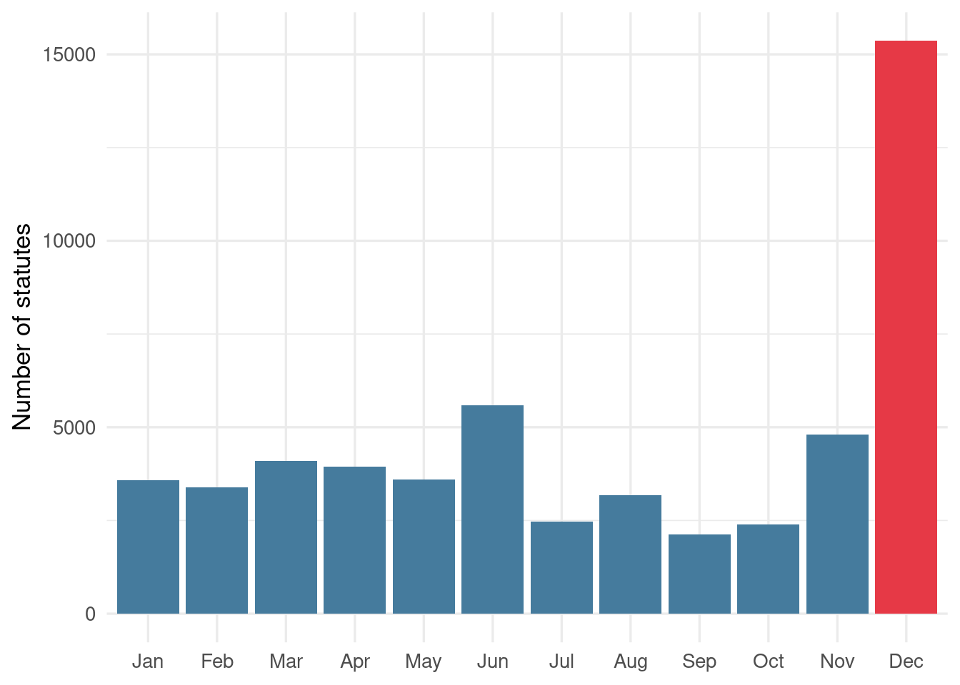
## Finding 3: Laws change fast, and December dominates
Two more questions fall out of the same data. First, how long does a law survive before its first amendment? Restricting to laws enacted from 1990 onward (so the full history is observed), the median time to first amendment is just **two years**, and nearly half of all laws are amended within two years of enactment. A law rarely stabilises before it is revised.
Second, *when* in the year are statutes issued?
```{r december}
month_data <- rik_a |>
  filter(!is.na(kuukausi)) |>
  count(kuukausi)
dec_share <- round(month_data$n[month_data$kuukausi == 12] / sum(month_data$n) * 100)
```
```{r december-plot}
#| fig-cap: "Statutes issued by month. December alone accounts for over a quarter of the year's legislation."
#| code-fold: true
month_names <- c("Jan","Feb","Mar","Apr","May","Jun",
                 "Jul","Aug","Sep","Oct","Nov","Dec")
month_data |>
  mutate(m = factor(month_names[kuukausi], levels = month_names)) |>
  ggplot(aes(m, n, fill = kuukausi == 12)) +
  geom_col(show.legend = FALSE) +
  scale_fill_manual(values = c(`FALSE` = "#457b9d", `TRUE` = "#e63946")) +
  labs(x = NULL, y = "Number of statutes") +
  theme_minimal(base_size = 13)
```
December accounts for `r dec_share`% of all statutes — a consequence of new rules timed to take effect at the turn of the year. The pattern is structural and holds across statute types, not just budget laws.
## Finding 4: Knowing what you cannot predict
A forecast is only worth making if the quantity has predictable structure. The annual *total* number of statutes does not: its year-to-year autocorrelation is essentially zero, so it is noise around a stable mean. Recognising this is itself a result — it prevents a misleading forecast.
The number of *new* statutes is different. It has strong autocorrelation and a clear downward trend. A Bayesian linear trend model on the log scale produces a genuinely informative forecast: new legislation is declining at roughly 2–3% per year, and the projection carries this forward with honest, and narrow, uncertainty bands. The substantive reading reinforces the whole analysis — legislative work is shifting from creating new law toward amending what already exists.
## Why this matters
None of these findings required privileged access or proprietary data. They came from a free public API, a few hundred lines of R, and statistical methods that quantify uncertainty rather than hide it. The same pipeline applies to any domain-specific question — the change rate of a single field of law, the volatility of statutes referenced in a contract, or a comparison of legislative turnover across sectors.
The barrier to this kind of analysis is technical, not legal. That is precisely where the collaboration between domain expertise and data science creates value that neither produces alone.
## Reproducing this analysis
The full retrieval and analysis code is available on request. The pipeline has four stages:
1. **Retrieve the statute list** — loop over years and categories against the Finlex REST API, keep Finnish-language URIs, paginate to exhaustion.
2. **Retrieve amendment targets** — for each amending and repealing statute, fetch its Akoma Ntoso XML and extract the `affectedDocument` reference. This is the long step (~35,000 requests).
3. **Enrich metadata** — fetch `dateIssued`, title, and section count per statute to derive month, statute type, and length.
4. **Analyse** — changepoint detection, change-frequency distribution, timing, and the Bayesian trend forecast.
Every stage caches to disk (`.fst` and `.rds`) so the expensive retrieval runs once. The analysis layer reads only local files, which keeps it fast and reproducible — and crucially, lets it run in a CI environment such as GitHub Actions without hitting the API.
---
*Kristian Vepsäläinen is an independent data scientist (M.Sc. mathematics, M.Eng. cyber security) specialising in open-data analysis, Bayesian methods, and turning public data into decision-relevant insight. [kristianvepsalainen.com](https://www.kristianvepsalainen.com)*